Generalised logistic function

From Quire, the open reference·Mathematical function·2 min read

Redirected from Generalized logistic function

Effect of varying parameter A. All other parameters are 1. Image: source and license

Effect of varying parameter B. A = 0, all other parameters are 1. Image: source and license

Effect of varying parameter C. A = 0, all other parameters are 1. Image: source and license

Effect of varying parameter K. A = 0, all other parameters are 1. Image: source and license

Effect of varying parameter Q. A = 0, all other parameters are 1. Image: source and license

Effect of varying parameter . A = 0, all other parameters are 1. — Effect of varying parameter ${\displaystyle \nu }$ . A = 0, all other parameters are 1. Image: source and license

The generalized logistic function or curve is an extension of the logistic or sigmoid functions. Originally developed for growth modelling, it allows for more flexible S-shaped curves. The function is sometimes named Richards's curve after F. J. Richards, who proposed the general form for the family of models in 1959.

Definition#edit

Richards's curve has the following form:

${\displaystyle Y(t)=A+{K-A \over (C+Qe^{-Bt})^{1/\nu$

where ${\displaystyle Y}$ = weight, height, size etc., and ${\displaystyle t}$ = time. It has six parameters:

${\displaystyle A}$ : the left horizontal asymptote;
${\displaystyle K}$ : the right horizontal asymptote when ${\displaystyle C=1}$ . If ${\displaystyle A=0}$ and ${\displaystyle C=1}$ then ${\displaystyle K}$ is called the carrying capacity;
${\displaystyle B}$ : the growth rate;
${\displaystyle \nu >0}$ : affects near which asymptote maximum growth occurs.
${\displaystyle Q}$ : is related to the value ${\displaystyle Y(0)}$
${\displaystyle C}$ : typically takes a value of 1. Otherwise, the upper asymptote is ${\displaystyle A+{K-A \over C^{\,1/\nu$

The equation can also be written:

${\displaystyle Y(t)=A+{K-A \over (C+e^{-B(t-M)})^{1/\nu$

where ${\displaystyle M}$ can be thought of as a starting time, at which ${\displaystyle Y(M)=A+{K-A \over (C+1)^{1/\nu$ . Including both ${\displaystyle Q}$ and ${\displaystyle M}$ can be convenient:

${\displaystyle Y(t)=A+{K-A \over (C+Qe^{-B(t-M)})^{1/\nu$

this representation simplifies the setting of both a starting time and the value of ${\displaystyle Y}$ at that time.

The logistic function, with maximum growth rate at time ${\displaystyle M}$ , is the case where ${\displaystyle Q=\nu =1}$ .

Generalised logistic differential equation#edit

A particular case of the generalised logistic function is:

${\displaystyle Y(t)={K \over (1+Qe^{-\alpha \nu (t-t_{0})})^{1/\nu$

which is the solution of the Richards's differential equation (RDE):

${\displaystyle Y^{\prime }(t)=\alpha \left(1-\left({\frac {Y}{K\right)^{\nu }\right)Y}$

with initial condition

${\displaystyle Y(t_{0})=Y_{0$

where

${\displaystyle Q=-1+\left({\frac {K}{Y_{0\right)^{\nu$

provided that ${\displaystyle \nu >0}$ and ${\displaystyle \alpha >0}$

The classical logistic differential equation is a particular case of the above equation, with ${\displaystyle \nu =1}$ , whereas the Gompertz curve can be recovered in the limit ${\displaystyle \nu \rightarrow 0^{+$ provided that:

${\displaystyle \alpha =O\left({\frac {1}{\nu \right)}$

In fact, for small ${\displaystyle \nu }$ it is

${\displaystyle Y^{\prime }(t)=Yr{\frac {1-\exp \left(\nu \ln \left({\frac {Y}{K\right)\right)}{\nu \approx rY\ln \left({\frac {Y}{K\right)}$

The RDE models many growth phenomena, arising in fields such as oncology and epidemiology.

Gradient of generalized logistic function#edit

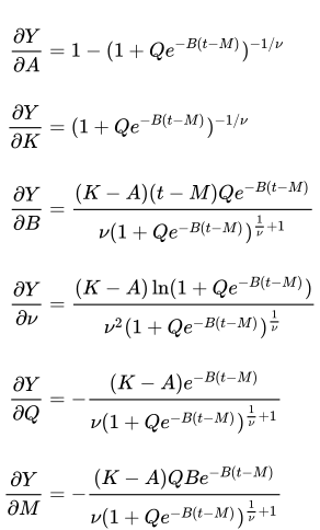
When estimating parameters from data, it is often necessary to compute the partial derivatives of the logistic function with respect to parameters at a given data point ${\displaystyle t}$ (see^[1]). For the case where ${\displaystyle C=1}$ ,

${\displaystyle {\begin{aligned}\\{\frac {\partial Y}{\partial A&=1-(1+Qe^{-B(t-M)})^{-1/\nu }\\\\{\frac {\partial Y}{\partial K&=(1+Qe^{-B(t-M)})^{-1/\nu }\\\\{\frac {\partial Y&#125$

Special cases#edit

The following functions are specific cases of Richards's curves:

Footnotes#edit

^ Fekedulegn, Desta; Mairitin P. Mac Siurtain; Jim J. Colbert (1999). "Parameter Estimation of Nonlinear Growth Models in Forestry" (PDF). Silva Fennica. 33 (4): 327–336. doi:10.14214/sf.653. Archived from the original (PDF) on 2011-09-29. Retrieved 2011-05-31.

References#edit

Richards, F. J. (1959). "A Flexible Growth Function for Empirical Use". Journal of Experimental Botany. 10 (2): 290–300. doi:10.1093/jxb/10.2.290.
Pella, J. S.; Tomlinson, P. K. (1969). "A Generalised Stock-Production Model". Bull. Inter-Am. Trop. Tuna Comm. 13: 421–496.
Lei, Y. C.; Zhang, S. Y. (2004). "Features and Partial Derivatives of Bertalanffy–Richards Growth Model in Forestry". Nonlinear Analysis: Modelling and Control. 9 (1): 65–73. doi:10.15388/NA.2004.9.1.15171.

This article is mirrored from “Generalised logistic function” on English Wikipedia, revision 1340005818, written by Wikipedia's contributors and licensed CC BY-SA 4.0. Editing it here creates a Quire copy with its own history.

Synced with Wikipedia revision 1340005818 · just now